Latent Iteractions in Structural Equation Models

I was eager to know how to modelling latent interactions for structural equation models in lavaan. There is this lavaan google group https://groups.google.com/forum/#!forum/lavaan where one can find a lot of comments by searching for “latent interactions”.  Basicly there is one paper from Mash (2004) and one from Lin (2010) explaining the methods in detail. Inspired by https://rpubs.com/mkearney/103098 (data not available) I compiled a script summarizing the methods developed by Marsh (2004) and Lin (2010) by using the HolzingerSwineford1939 data.

See  http://rpubs.com/candrea/latintsem .


Recursive R function to find intersection of two or more given sets

The intersect(x, y) function from R “base” package works for no more then two vectors x and y.  The following function accepts as many vectors as you like and returns the intersection vector of them all:

## recursive intersect function
intersect.rec <- function(x, ...) {
    a <- list(...)
    if(length(a) == 0) stop("Two or more arguments are needed.")
    if(is.list(a[[1]])) a <- a[[1]]
    if(length(a) == 1) return(intersect(x, a[[1]]))
    else intersect.rec(intersect(x, a[[1]]), a[-1])
}

Sample usage:

x <- letters[1:5]
y <- letters[2:5]
z <- letters[3:5]
intersect.rec(x, y, z)
## returns
## [1] "c" "d" "e"

This is especially a basic example of an R function using dots argument and recursively iterating over them.

CFA with a single factor

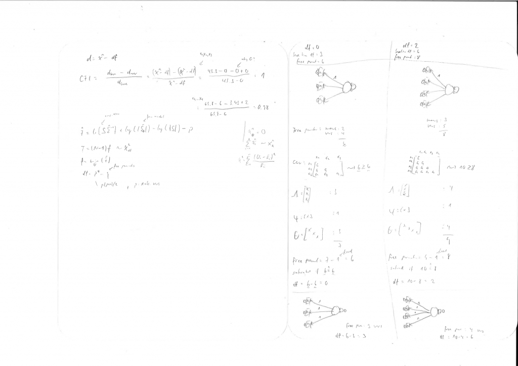
Fit values for a CFA with a single factor can only be computed with models with more than 3 observed variables. With 3 obeserved variables and one factor you have to compute 6 free parameters (with one fixed). But your covariance matrix has also 6 nonredundant elements. Hence you get df=0 degress of freedom. A chi-squared distribution with df=0 is constant 0, hence we can expect the test statistic to be 0.

CFA single factor

20151216121756

Little letters are also important

In the PISA 2012 Technical Report on page 312 (chapter 16), the formula (16.3) for the Partial Credit Model is printed for computing scale parameters. Looking at it twice, one can see that something must be wrong with the subscribs used for the sumations.

P_{x_i}(\theta_n) = \frac{\displaystyle\exp\sum_{k=0}^x(\theta_n-\delta_i+\tau_{ij})}{\displaystyle\sum_{h=0}^{m_i}\exp\displaystyle\sum_{k=0}^h(\theta_n-\delta_i+\tau_{ik})}


By consulting the chapter “Polytomous Rasch Models and their Estimation” in the book “Rasch Models” (Fischer, 1995), and combining the formulas (15.3) with (15.8) there, we get

P(X_{vi}=h) = \frac{\displaystyle\exp(\phi_h\theta_v + \sum_{l=0}^{h}\alpha_{il})}{\displaystyle\sum_{l=0}^m \exp(\phi_h\theta_v + \sum_{j=0}^{l}\alpha_{ij})}


Now by comparing the meaning of all the symbols and applying it on the formula from PISA Technical Report – by respecting as much as possible of the notations used by them – we get

P_{x_i}(\theta_n) = \frac{\displaystyle\exp\sum_{k=0}^{x_i}(\theta_n-\delta_i+\tau_{ik})}{\displaystyle\sum_{h=0}^{m_i}\exp\displaystyle\sum_{k=0}^h(\theta_n-\delta_i+\tau_{ik})}


We see that we have to change \tau_{ij} in the numerator of the very first formula above to \tau_{ik}, and x to x_i.

That makes sense!

A Simple Method of Sample Size Calculation for Logistic Regression

This posting is based on the paper “A simple method of sample size calculation for linear and logistic regression” by F. Y. Hsieh et al., which can be found under http://dx.doi.org/10.1002/(SICI)1097-0258(19980730)17:14<1623::AID-SIM871>3.0.CO;2-S .

We consider  the case where we want to calculate the sample size for a multiple  logistic regression with continous response variable and with continous covariates.

Fomula (1) in the paper computes the required sample size for a simple logistic regression, given the effect size to be tested, the event rate at the mean of the (single) covariate, level of significance, and required power for the test. This formula is implemented in the function SSizeLogisticCon()  from R package “powerMediation” and can easily be applied.

For the multiple case, Hsieh et al. introduce the variance inflation factor (VIF), with which the sample size for the simple case can be inflated to get the sample size for the multiple case. I have implemented it as R function:

## p1: the event rate at the mean of the predictor X
## OR: expected odds ratio. log(OR) is the change in log odds 
##     for an increase of one unit in X.
##     beta*=log(OR) is the effect size to be tested
## r2: r2 = rho^2 = R^2, for X_1 ~ X_2 + ... + X_p
ssize.multi <- function(p1, OR, r2, alpha=0.05, power=0.8) {
	n1 <- SSizeLogisticCon(p1, OR, alpha, power)
	np <- n1 / (1-r2)
	return(np)
}

Another approximation for the simple case is given in Formula (4), and is based on formulae given by A. Whittemore in “Sample size for logistic regression with small response probability”. I have implemente the simple case,

## p1: as above
## p2: event rate at one SD above the mean of X
ssize.whittemore <- function (p1, p2, alpha = 0.05, power = 0.8) {
    beta.star <- log(p2*(1-p1)/(p1*(1-p2)))
    za <- qnorm(1 - alpha/2)
    zb <- qnorm(power)
    V0 <- 1
    Vb <- exp(-beta.star^2 / 2)
    delta <- (1+(1+beta.star^2)*exp(5*beta.star^2 / 4)) * (1+exp(-beta.star^2 / 4))^(-1)
    n <- (V0^(1/2)*za + Vb^(1/2)*zb)^2 * (1+2*p1*delta) / (p1*beta.star^2)
    n.int <- ceiling(n)
    return(n.int)
}

and the multiple case.

## all parameters as above
ssize.whittemore.multi <- function(p1, p2, r2, alpha=0.05, power=0.8) {
	n1 <- ssize.whittemore(p1, p2, alpha, power)
	np <- n1 / (1-r2)
	return(np)
}

The complete R script, the examples from the paper included, can be found under http://rpubs.com/candrea/ssizelogreg .
 

New R Package “betas”

In social science it is often required to compute standardized regression coefficients – called beta coefficients, or simply betas. These betas can be interpreted as effects, and thus are independent of the original scale.

There are two approaches how you can obtain betas. You Z-standardize the data before fitting or you compute the betas after fitting the model.

The first approach has flaws if you have non-numeric variables in your data or if you intent to incorporate interaction terms in your model.

The second approach is a way more convenient, but until now there was no R package helping you compute betas for as many kinds of models as you needed. For example with lm.beta() from “QuantPsyc” Package you cannot handle models with factors with more than two levels.

The features of the “betas” R package are (so far for v0.1.1):

Compute standardized beta coefficients and corresponding standard errors for the following models:

  • linear regression models with numerical covariates only
  • linear regression models with numerical and factorial covariates
  • weighted linear regression models
  • all these linear regression models with interaction terms
  • robust linear regression models with numerical covariates only

You can install the package from CRAN (http://cran.r-project.org/web/packages/betas/):

install.packages("betas")
library(betas)

The package is maintained on GitHub: https://github.com/andreaphsz/betas .

Feel free to report issues: https://github.com/andreaphsz/betas/issues .

Enjoy hassle-free computations of betas in R!

Robust Standardized Beta Coefficients

Standardized beta coefficients are definded as

beta = b * sd_x/sd_y

where b are the coefficients from OLS linear regression, and sd_x and sd_y are standard deviations of each x variable and of y.

In the case where you performe a robust linear regression, sd_x and sd_y seems not be very meanigfull anymore, because variances and hence standard deviations are not robust. The R package “robust” provides the function covRob() to compute a robust covariance estimator.

I have written the following function to compute standardized beta coefficients for a robust linear regression. Setting the parameter classic=TRUE gives you the classic estimation of the beta coefficients. For very bad data, the covRob() function cannot compute the covariance due singularities. In this case the classical estimator is returned.

my.lmr.beta <- function (object, classic = FALSE) {
  if(class(object) != "lmRob")
    stop("Object must be of class 'lmRob'")
  model <- object$model
  num <- sapply(model, is.numeric)  # numeric vars only
  b <- object$coefficients[num][-1]  # final coefficients w/o intercept
  ## compute robust covariance
  covr <- NULL
  try(covr <- diag(covRob(model[num])$cov), silent = TRUE)
  if(is.null(covr) & classic == FALSE)
    warning("covRob() coud not be computed, instead covClassic() was applied.")
  ## compute classic covariance if robust failed
  if(is.null(covr) | classic == TRUE)
    covr <- diag(covClassic(model[num])$cov)
  sx <- sqrt(covr[-1])  # standard deviation of x's
  sy <- sqrt(covr[1])  # standard deviation of y
  beta <- b * sx/sy
  return(beta)
}

 UPDATE — 2014-07-23

Computing standard deviations for factors makes sense, because variance is definded for the binomial distribution.  So I have removed the num variable.

my.lmr.beta <- function (object, classic = FALSE) {
  if(class(object) != "lmRob")
    stop("Object must be of class 'lmRob'")
  model <- object$model
  #num <- sapply(model, is.numeric)  # numeric vars only
  b <- object$coefficients[-1]  # final coefficients w/o intercept
  ## compute robust covariance
  covr <- NULL
  try(covr <- diag(covRob(model)$cov), silent = TRUE)
  if(is.null(covr) & classic == FALSE)
    warning("covRob() coud not be computed, instead covClassic() was applied.")
  ## compute classic covariance if robust failed
  if(is.null(covr) | classic == TRUE)
    covr <- diag(covClassic(sapply(model, as.numeric))$cov)
  sx <- sqrt(covr[-1])  # standard deviation of x's
  sy <- sqrt(covr[1])  # standard deviation of y
  beta <- b * sx/sy
  return(beta)
}


Select Pupils by Number of Pupils per Group

Selecting rows conditioned on values in columns is easy, as for example selecting people aged over 33. What is about selecting rows conditioned on statistics computed on multiple rows of the data frame, as for example selecting pupils in groups by the number of pupils per group?

That is where the very nice dplyr package comes in.

We build and print the data frame:

df <- data.frame(id=1:9, classid=c(1,1,1,2,2,3,3,3,3), math=round(runif(9,1,6),1))
> print(df)
  id classid math
1  1       1  5.4
2  2       1  4.0
3  3       1  1.1
4  4       2  2.2
5  5       2  3.9
6  6       3  2.7
7  7       3  6.0
8  8       3  2.0
9  9       3  1.6

Now, we want to select – i.e. “filter” in terms of the dplyr package – pupils that are part of groups/classes with more than two pupils per class. In dplyr there are three different syntaxes to achieve this.

# step-by-step
df.g <- group_by(df, classid)
df.n <- filter(df.g, n()>2)

# or nested syntax
df.n <- filter(group_by(df, classid), n()>2)

# or with %.% operator
df.n <- df %.% 
  group_by(classid) %.% 
  filter(n()>2)

The result is the same for all:

> print(df.n)
Source: local data frame [7 x 3]
Groups: classid

  id classid math
1  1       1  5.4
2  2       1  4.0
3  3       1  1.1
4  6       3  2.7
5  7       3  6.0
6  8       3  2.0
7  9       3  1.6

Of course, you can do this the pure-R-way,

> df.c <- df[df$classid %in% which(xtabs(~classid, df)>2), ]
> print(df.c)
  id classid math
1  1       1  5.4
2  2       1  4.0
3  3       1  1.1
6  6       3  2.7
7  7       3  6.0
8  8       3  2.0
9  9       3  1.6

but I think with dplyr it looks quite a bit nicer.

Happy dpylr!

Installing JAGS 3.4.0 under OS X 10.9 Maverick

First of all see the excellent installation manual by Martyn Plummer and Bill Northcott (JAGS Version 3.4.0 installation manual) at section 2 “Mac OS X”.

For the rest of us (me included) thinking  ./configure without any options will do the job are getting the following error:

configure: error: "You need to install the LAPACK library"

(It will not work even with the  –with-lapack=’-framework vecLib’ option.)

Do not follow this instruction! You do not have to install the LAPACK library because on OS X 10.9 the optimized (accelerated by Apple engineers) version of LAPACK is allready installed, see the LAPACK(7) Mac OS X Manual Page.

From now on just type the slightly modified commands in your bash-shell (terminal):

export CC=/usr/bin/clang

export CXX=/usr/bin/clang++

export CFLAGS="-g -Os -mmacosx-version-min=10.6 -isysroot /Applications/Xcode.app/Contents/Developer/Platforms/MacOSX.platform/Developer/SDKs/MacOSX10.9.sdk -arch i386 -arch x86_64"

export CXXFLAGS="-g -Os -mmacosx-version-min=10.6 -isysroot /Applications/Xcode.app/Contents/Developer/Platforms/MacOSX.platform/Developer/SDKs/MacOSX10.9.sdk -arch i386 -arch x86_64"

export FFLAGS="-g -Os -mmacosx-version-min=10.6 -isysroot /Applications/Xcode.app/Contents/Developer/Platforms/MacOSX.platform/Developer/SDKs/MacOSX10.9.sdk -arch i386 -arch x86_64"

export LDFLAGS="-mmacosx-version-min=10.6 -arch i386 -arch x86_64"

./configure --disable-dependency-tracking --with-included-ltdl

make -j 8

sudo make install

Of course, make sure you have installed all the required tools before executing the commands.

Happy ./configuring!